Projections

In this exercise, I explored the results of using various projections in ArcGIS Pro and compared the resulting calculated areas of several Florida counties. First, I acquired the data needed for this project; one file was available through the GIS student repository, while the other was downloaded from FGDL.org. Then, I had my first introduction to the ArcGIS Pro Geoprocessing Tools. I used the Project Tool to create two new maps by changing the projection systems. The original map utilizes Albers, while the newly created maps utilize UTM 16 and Florida State Plane North. Then, I utilized attributes table to compare the projections quantitatively. To do this, I first used the Geoprocessing tool Calculate Geometry Attributes to create a calculation for polygonal area of each county in square miles. Once this was done, I opened the attributes tables of each projection and created new layers to isolate the counties of Polk, Miami-Dade, Escambia, and Alachua. Interestingly, each projection method resulted in different area calculations for these counties. I transferred the information into an Excel table for better analysis.
This exercise demonstrates how critical it is to keep projections consistent throughout a project in order to conduct accurate, viable area comparisons, as we can see that calculated area varies greatly among projection methods. Here, the results between Albers and State Plane N are fairly similar to one another, while the results of UTM 16 N are much further outliers. According to the U.S. Census Bureau, the actual areas of these counties are as follows: Alachua being 969 square miles, Escambia being 875 square miles, Miami-Dade being 2431 square miles, and Polk being 2010 square miles. It is challenging to determine which projection is best, as all three have significantly distorted the county areas. Both Albers and State Plane N work well with Alachua County and Polk County. Meanwhile, all three offered poor calculations for the areas of Escambia and Miami-Dade. This seems to indicate that the projections maintain the greatest accuracy for the center of the state, where Alachua and Polk are located, but loses quality significantly in areas on the state’s periphery, as Escambia and Miami-Dade are.
Finally, I designed a layout to show each map side-by-side. I was careful to include all essential map elements, including title, preparer, data sources, legend, north arrow, and scale bar. In addition to these things, I included the table demonstrating the areas calculated within each projection. When designing the layout, I used guides and neatlines to separate the area into quadrants, so three could be used for projection maps and the fourth could be used to communicate general information. I made each county a unique color, and kept this consistent throughout the three maps. Hopefully, the result is an effective visual and quantitative comparison.
Comments
Post a Comment